If you’re responsible for wastewater treatment plant operations and haven’t quantified your aeration energy savings potential using actual oxygen transfer efficiency data, significant cost savings are likely slipping through your fingers. As a process engineer specializing in energy efficiency optimization, I’ve reviewed dozens of aeration system audits where facilities consumed 30-50% more energy than necessary—not from equipment failures, but from unoptimized operational parameters and outdated performance assumptions.
Most energy reduction guides miss this critical reality: aeration optimization requires a layered approach where each tier delivers diminishing but cumulative returns. I’ll demonstrate the data-driven framework that has achieved 40-70% energy reductions across multiple facilities, complete with calculation tools and implementation strategies that transform theoretical savings into measurable results.
Understanding Aeration Energy Consumption: The Data Behind the Problem
First, establish what we’re optimizing against. The commonly cited statistic—aeration consumes 40-60% of total wastewater treatment plant energy—is accurate but incomplete. The crucial insight lies in understanding why this percentage varies so widely and how specific technical parameters determine your facility’s energy consumption profile.
The Oxygen Transfer Efficiency (OTE) Reality Gap
Significant gaps exist between theoretical and actual oxygen transfer efficiency at most facilities. Equipment specifications show Standard Oxygen Transfer Efficiency (SOTE) values—typically 20-55% for fine bubble diffusers and 5-25% for coarse bubble diffusers—representing clean water testing under ideal conditions. Actual wastewater treatment applications reduce these values through several adjustment factors:
- Alpha factor (α): 0.4-0.9 depending on bubble size and wastewater contaminants
- Beta factor (β): 0.95 at 20°C decreasing to 0.78 at 30°C
- Salinity impact:
SOTE_adj = SOTE × (1 - 0.006 × Salinity_ppt)
Applying these adjustments reveals that a fine bubble diffuser with 40% clean water SOTE typically delivers only 20-28% effective SOTE in field conditions. This efficiency gap directly translates to energy waste: facilities supply more air than necessary to achieve required oxygen transfer.
Energy Consumption Benchmarks: What Good Looks Like
Establish realistic optimization targets with these industry energy consumption benchmarks:
Fine Bubble Diffusers:
- Energy consumption: 0.45-0.65 kWh/kg O₂ transferred
- Oxygen transfer rate: 4.5-6.2 kg O₂/kWh
- This represents the efficiency ceiling for most municipal applications
Coarse Bubble Diffusers:
- Energy consumption: 1.2-1.8 kWh/kg O₂ transferred
- Oxygen transfer rate: 1.2-1.8 kg O₂/kWh
- Typically used where mixing requirements outweigh oxygen transfer efficiency needs
The 2.5-3x energy consumption difference between these technologies isn’t theoretical—it’s measurable and significant for facilities processing millions of gallons daily. But equipment selection is just one component of the optimization equation.
The Three-Tiered Framework for Aeration Energy Reduction
Analysis of dozens of optimization projects reveals a framework that structures energy reduction strategies into three tiers, each with distinct characteristics:
| Tier | Strategy | Typical Energy Savings | Implementation Complexity | Capital Cost | Key Success Factors |
|---|---|---|---|---|---|
| Tier 1 | Operational Optimization (Low DO) | 25-60% | Medium | Low to Medium | Advanced controls, monitoring, operator training |
| Tier 2 | Equipment Efficiency Upgrades | 20-40% | High | High | Proper technology selection, installation quality |
| Tier 3 | Advanced Control Systems | 15-30% | High | Medium to High | Sensor accuracy, algorithm tuning, integration |
The critical insight from this framework: savings accumulate but implementation should proceed sequentially. Start with Tier 1 optimizations (highest ROI), then progress to Tiers 2 and 3 as budget and operational readiness allow. Attempting all three simultaneously often leads to implementation failures and underestimated complexity.
Why This Framework Beats Piecemeal Approaches
Most facilities approach energy reduction reactively—addressing obvious inefficiencies without a systematic plan. This leads to:
- Suboptimal sequencing: Investing in expensive equipment before optimizing operations
- Missed synergies: Failing to leverage how control systems enhance both operational and equipment efficiency
- Unrealized potential: Stopping after initial savings without pursuing cumulative benefits
The three-tiered framework addresses these pitfalls by providing a logical progression that maximizes total savings while managing implementation risk.
Tier 1: Operational Optimization Through Low DO Strategies
Operational optimization delivers the highest return on investment because it requires minimal capital expenditure while addressing the most common source of energy waste: over-aeration. Most wastewater treatment plants operate at dissolved oxygen (DO) concentrations higher than necessary for effective treatment.
The Science Behind Low DO Operations
The relationship between DO concentration and energy consumption isn’t linear—it’s exponential. As DO setpoints decrease, the driving force for oxygen transfer decreases, requiring less air flow to maintain the same oxygen transfer rate. However, there’s a critical threshold where biological processes become oxygen-limited.
Optimal DO Ranges by Process:
- Conventional activated sludge: 1.0-2.0 mg/L (often operated at 2.5-4.0 mg/L)
- Nitrification systems: 0.8-1.5 mg/L (maintaining nitrification while minimizing energy)
- MBBR/IFAS systems: 1.5-3.0 mg/L (accounting for biofilm diffusion limitations)
The key is identifying your facility’s minimum effective DO through gradual reduction and performance monitoring, not adopting generic targets.
Case Study Evidence: Real-World Savings from Low DO Implementation
Pomona Water Reclamation Plant:
- Reduced aeration energy from 1,300 kWh/MG to 550 kWh/MG (60% reduction)
- Implemented ammonia-based aeration control with machine learning algorithms
- Maintains nitrification at DO concentrations below 1 mg/L
- Key insight: Advanced control algorithms enabled lower DO operation without compromising treatment quality
City of St. Cloud’s NEW Recovery Facility:
- Transitioned from 2.5 mg/L DO to below 0.8 mg/L DO
- Achieved 30% energy savings through phased implementation
- Key insight: Gradual reduction allowed operators to adjust to new operating parameters
Boxelder Sanitation District:
- Achieved 25% aeration energy reduction through low DO optimization
- Key insight: Even facilities without advanced controls can achieve significant savings through manual optimization
Implementation Guidelines for Low DO Operations
- Baseline establishment: Measure current DO profiles and energy consumption
- Gradual reduction: Lower DO setpoints by 0.2-0.5 mg/L increments weekly
- Performance monitoring: Track nitrification rates, effluent ammonia, and sludge settling
- Threshold identification: Determine the minimum DO that maintains treatment objectives
- Control optimization: Implement DO control strategies (cascade, feedforward, model-based)
The most common mistake in low DO implementation is rushing the process. Biological systems need time to adapt to new oxygen conditions, and operators need time to build confidence in the new operating regime.
Tier 2: Equipment Efficiency Through Diffuser and Blower Upgrades
Once operational optimization is maximized, equipment upgrades provide the next layer of energy savings. This tier involves replacing or upgrading aeration system components to improve oxygen transfer efficiency.
Fine Bubble vs. Coarse Bubble: The Data-Driven Comparison
| Parameter | Fine Bubble Diffusers | Coarse Bubble Diffusers | Practical Implications |
|---|---|---|---|
| Bubble Size | 1-3 mm | 4-20 mm | Fine bubbles create more surface area for oxygen transfer |
| SOTE Range | 20-55% | 5-25% | Field conditions typically reduce these values by 30-50% |
| Energy Consumption | 0.45-0.65 kWh/kg O₂ | 1.2-1.8 kWh/kg O₂ | Fine bubble saves 40-65% on energy costs |
| Oxygen Transfer Rate | 4.5-6.2 kg O₂/kWh | 1.2-1.8 kg O₂/kWh | |
| Mixing Capability | Moderate | Excellent | Coarse bubble better for high solids applications |
| Fouling Resistance | Lower | Higher | Coarse bubble requires less maintenance |
| Service Life | 3-5 years | 5-8+ years | Depends on membrane material and wastewater characteristics |
| Initial Cost | Higher | Lower | Coarse bubble is 25-40% cheaper initially |
| Operating Cost | Lower | Higher | Fine bubble energy savings offset higher initial cost |
Application-Specific Technology Selection
The “best” diffuser technology depends on your specific application requirements:
Fine bubble diffusers with high-quality EPDM membranes are optimal when:
- Oxygen transfer efficiency is the primary concern
- Wastewater has low fouling potential
- Energy costs are high relative to capital budget
- The facility can accommodate periodic membrane replacement
Fine bubble tube diffusers offer advantages for:
- Channels with high flow velocities (better resistance to shear forces)
- Applications requiring uniform oxygen distribution along length
- Facilities with space constraints for diffuser placement
Coarse bubble diffusers are preferable when:
- Mixing requirements outweigh oxygen transfer needs
- Wastewater has high fouling potential (grease, fibers, etc.)
- Maintenance access is limited
- Capital budget constraints prioritize lower initial cost
Lifecycle Cost Analysis: The Real Decision Metric
Equipment selection should be based on total lifecycle cost, not just initial capital expenditure. Consider this example:
Scenario: 10 MGD facility with $0.10/kWh energy cost
- Fine bubble upgrade: $500,000 capital cost, 0.55 kWh/kg O₂ energy consumption
- Coarse bubble replacement: $300,000 capital cost, 1.5 kWh/kg O₂ energy consumption
- Annual oxygen demand: 10,000 kg O₂/day
Annual Energy Cost Comparison:
- Fine bubble: 10,000 kg/d × 0.55 kWh/kg × 365 d × $0.10/kWh = $200,750
- Coarse bubble: 10,000 kg/d × 1.5 kWh/kg × 365 d × $0.10/kWh = $547,500
Simple Payback for Fine Bubble Upgrade:
- Additional capital: $200,000
- Annual savings: $346,750
- Payback period: 0.58 years (7 months)
This analysis explains why fine bubble upgrades often have surprisingly short payback periods despite higher initial costs. For integrated biofilm systems where aeration optimization complements MBBR media performance, our data-driven guide to MBBR media selection provides coordinated optimization strategies.
Case Study: Fine Bubble Membrane Upgrade Results
Fine Bubble Upgrade Results:
- 28.3% energy savings achieved
- 63.9% higher Oxygen Transfer Efficiency (OTE)
- Payback period of 1.8 years despite significant capital investment
- Key insight: The efficiency improvement more than justified the upgrade cost
Tier 3: Advanced Control Systems for Precision Aeration
The third tier involves implementing sophisticated control strategies that optimize aeration in real-time based on process conditions. While this tier provides the smallest incremental savings percentage, it optimizes the performance of both Tier 1 and Tier 2 improvements.
Control Strategy Options and Applications
Ammonia-Based Aeration Control (ABAC):
- Uses online ammonia sensors to adjust aeration based on actual nutrient removal needs
- Particularly effective for plants with variable loading
- Can reduce aeration by 15-25% compared to DO-based control
Model Predictive Control (MPC):
- Uses mathematical models to predict oxygen demand and optimize aeration
- Requires significant tuning and validation
- Can achieve 20-30% additional savings over conventional control
Artificial Intelligence/Machine Learning:
- Learns patterns from historical data to optimize aeration
- Adapts to changing conditions without manual retuning
- Demonstrated 15-20% savings in pilot applications
Case Study: AI-Optimized Aeration in Rennes, France
AI-Optimized Aeration Results:
- 15% reduction in aeration costs
- 1,200 MWh reduction in energy consumption annually
- 41 tons of CO₂ avoided annually
- Key insight: Advanced controls provided savings beyond what was achievable through equipment upgrades alone
Implementation Considerations for Advanced Controls
- Sensor reliability: Advanced controls depend on accurate, reliable sensors
- Algorithm tuning: Most systems require significant site-specific tuning
- Operator training: New control strategies require different operator skills
- Integration complexity: Must work with existing SCADA and control systems
- Maintenance requirements: More sophisticated systems often have higher maintenance needs
The most successful advanced control implementations start with pilot testing on a single basin or treatment train before plant-wide deployment.
Calculating Your Savings Potential: A Step-by-Step Framework
Translate these strategies into actionable plans by quantifying potential savings for your specific facility. Here’s a complete calculation framework:
Step 1: Calculate Standard Oxygen Requirement (SOR)
SOR = [Q_w × (BOD₅/δ) × 1.2 + 4.6 × N_k - 2.6 × N_d] × K_tWhere:
Q_w= Daily treatment water volume (m³/d)BOD₅= Five-day biochemical oxygen demand (mg/L)N_k= Nitrification ammonia nitrogen amount (kg/d)N_d= Denitrification nitrogen removal amount (kg/d)K_t= Temperature correction coefficient
Step 2: Determine Required Air Flow
Q_air = SOR / (0.21 × ρ_O₂ × E) × 1.2Where:
0.21= Oxygen content in airρ_O₂= Oxygen density = 1.43 kg/m³E= Aerator oxygen utilization rate (adjusted SOTE)1.2= Safety factor
Step 3: Calculate Energy Consumption
Energy (kWh/d) = Q_air × P_specific × 24 / η_blowerWhere:
P_specific= Specific power consumption of blower (kW/m³/s)η_blower= Blower efficiency (typically 0.7-0.85)
Step 4: Estimate Savings by Tier
Tier 1 Savings (Low DO):
Savings_T1 = Current_Energy × (0.25 to 0.60) × Implementation_FactorTier 2 Savings (Equipment Upgrade):
Savings_T2 = Current_Energy × (0.20 to 0.40) × Technology_FactorTier 3 Savings (Advanced Controls):
Savings_T3 = (Current_Energy - Savings_T1 - Savings_T2) × (0.15 to 0.30)Worked Example: 5 MGD Municipal Plant
Current Conditions:
- Flow: 5 MGD (18,927 m³/d)
- Energy consumption: 1,800,000 kWh/year
- Current SOTE: 18% (coarse bubble, aged)
- Energy cost: $0.12/kWh
Optimization Potential:
- Tier 1 (Low DO): 30% savings = 540,000 kWh/year = $64,800/year
- Tier 2 (Fine bubble upgrade): 35% savings = 630,000 kWh/year = $75,600/year
- Tier 3 (Advanced controls): 15% of remaining = 94,500 kWh/year = $11,340/year
Total Potential Savings:
- Energy: 1,264,500 kWh/year (70% reduction)
- Cost: $151,740/year
- CO₂ reduction: ~900 metric tons/year (assuming 0.7 kg CO₂/kWh)
Your Implementation Roadmap: From Assessment to Validation
Successful aeration energy reduction requires systematic implementation. Follow this phased approach to maximize success while minimizing risk:
Phase 1: Assessment and Baseline (Weeks 1-4)
- Analyze current energy consumption: Determine aeration’s percentage of total plant energy
- Measure actual SOTE/OTE: Conduct field testing to establish baseline efficiency
- Evaluate DO control effectiveness: Review historical DO data and control strategies
- Assess diffuser condition: Inspect and document current diffuser performance
- Analyze energy cost structure: Understand time-of-use rates and demand charges
Phase 2: Planning and Prioritization (Weeks 5-8)
- Set energy reduction targets: Establish realistic percentage and cost savings goals
- Evaluate strategy applicability: Determine which tiers are feasible for your facility
- Calculate potential ROI: Use the framework above to quantify savings potential
- Develop phased implementation plan: Sequence Tier 1 → Tier 2 → Tier 3
- Identify risks and mitigation: Address potential treatment quality impacts
Phase 3: Implementation (Months 3-12)
- Start with Tier 1 optimizations: Implement low DO strategies for quick wins
- Optimize existing equipment: Maximize performance of current diffusers/blowers
- Plan Tier 2 upgrades: Design and budget for equipment improvements
- Implement Tier 3 controls: Pilot advanced control strategies
- Train operations staff: Ensure operators understand new strategies
Phase 4: Validation and Continuous Improvement (Ongoing)
- Monitor energy consumption changes: Track actual vs. projected savings
- Verify treatment performance: Ensure optimization doesn’t compromise effluent quality
- Calculate actual ROI: Compare implemented costs to achieved savings
- Document lessons learned: Create institutional knowledge for future projects
- Plan next optimization cycle: Identify additional improvement opportunities
Key Principles for Sustainable Energy Reduction
Based on my experience with dozens of optimization projects, these principles separate successful implementations from disappointing ones:
- Measure before optimizing: Without accurate baseline data, you can’t quantify improvements or identify the most promising opportunities.
- Prioritize operational changes before capital investments: The highest ROI strategies typically involve optimizing what you already have rather than buying new equipment.
- Consider total lifecycle costs: Equipment decisions should be based on 10-20 year cost projections, not just initial capital expenditure.
- Implement gradually and monitor closely: Biological systems need time to adapt to changes. Monitor key parameters to ensure treatment quality isn’t compromised.
- Engage operations staff early and often: Operators who understand the “why” behind changes are more likely to maintain optimized conditions.
- Validate savings with actual data: Don’t rely on theoretical calculations—measure actual energy consumption before and after implementation.
- View optimization as continuous, not one-time: The most successful facilities establish ongoing monitoring and adjustment processes.
Aeration energy optimization isn’t about finding a single magic solution—it’s about systematically addressing inefficiencies across operations, equipment, and controls. By following this three-tiered framework and implementation roadmap, you can achieve 40-70% energy reductions while maintaining or improving treatment performance.
The data shows the potential is real, the methodologies are proven, and the financial returns are substantial. The question isn’t whether you should optimize your aeration energy consumption, but how soon you can start implementing these strategies.